In order to find out if CAPE is present, and if so, how much, one can use a thermodynamic diagram. A thermodynamic diagram usually shows isotherms and isobars. Additionally it contains lines of equal…

potential temperature, called isentropes or dry adiabats

pseudo-potential temperature called pseudo-isentropes or moist adiabats, and

saturation mixing ratio rs, the isohumes.

Every air-parcel can be represented by two points in the diagram: one that depicts its temperature and pressure, and one that represents its moisture content and pressure. The vertical profiles of temperature and moisture data observed by radiosondes can be plotted on it as two curves.

A parcel of air that is not saturated with water vapour will conserve its potential temperature. It will always move along an isentrope in a thermodynamic diagram. When a saturated parcel rises -a process during which condensation takes place- its pseudo-equivalent potential temperature is conserved. Hence, it will move along a pseudo-isentrope in the diagram. For downward moving parcels that contain liquid water or ice, neither is true in general.

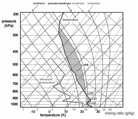
Fig. 1.1. Skew-T log p thermodynamic diagram, on which temperature and dew point temperature data from a radiosonde ascent are plotted. The diagram shows isobars, isotherms, lines of equal potential temperature theta (isentropes or dry adiabats), lines of equal pseudo-equivalent potential temperature theta-ep (pseudo-isentropes or moist adiabats) and lines of equal mixing ratio r (isohumes). An ascent curve T(p) of a parcel from the surface having an initial temperature of 26°C and a dew point temperature of 21°C has been constructed.

Figure 1.1 is a so-called skew-T, log-p thermodynamic diagram. To see if a parcel has CAPE, we construct the curve T(p) that the parcel would follow if it were lifted. It initially follows a curve parallel to the isentropes up to the level at which condensation takes place, the lifted condensation level (LCL), and follows a curve parallel to the pseudo-isentropes thereafter. In figure 1, the ascent curve of a parcel having a surface temperature of 27 C and a dew-point temperature of 21 C (corresponding with a mixing ratio of 15.5 g/kg) has been constructed. The LCL is found at the altitude where the mixing ratio of the parcel becomes equal to its the saturation mixing ratio. The saturation mixing ratio decreases as the parcel becomes colder during the ascent.

From the figure, one can see the difference between the parcel's temperature and that of its environment if the parcel were lifted. The altitude at which the parcel becomes less dense than its environment is the level of free convection (LFC). This roughly coincides with the level where it gets warmer than its environment. The level at which it ultimately becomes colder than its environment is called the equilibrium level (EL).

In a Skew-T, log-p diagram, the amount of CAPE is proportional to the surface area between the T(p) curve of the parcel and that of its environment bounded by the LFC and the EL (dark shaded in fig. 1.1). Computer programs can calculate the exact value of CAPE by performing a numerical integration of

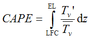
where Tv' is the difference between the (virtual) temperature of the parcel with it's environment and Tv'_bar is the average of the two.

In order for CAPE to be present, it is required that at some level in the troposphere, the lapse rates are steeper than the moist adiabatic lapse rate. Additionally, there must be enough moisture present below that level that a parcel can become warmer than its environment when it is lifted. Hence, an increase in CAPE is associated with one or more of the following processes:

an increase of low-level humidity

an increase of low-level temperature

a decrease of temperature in the mid- (or upper) troposphere

Often, a parcel has to ascend through a layer of air that is warmer than itself before it reaches its LFC. This layer is often colloquially called the cap. In other words, a parcel would need some "push" to get through such a layer: it has to contain some kinetic energy. The energy required to pass it, is called convective inhibition or CIN. If CIN is large, convection will likely not develop. CIN can be seen on the diagram as the area between the T(p) curve of the parcel and that of its environment below the LFC. More than 100 to 200 J/kg of CIN is usually too large to be overcome, even when strong thermals are present in the boundary layer below. The same processes that were mentioned above that increase CAPE have the effect to reduce CIN. A decrease of temperature at mid-level however has only effect as it occurs in the warm layer that inhibits convection for it to reduce CIN.